Augmenting Medical Images: Chest X-ray 14 dataset

In this notebook, we will show how to easily use SOLT for object detection tasks (actually finding detection) in medical imaging. First, we will use a low-level API to show how to create bounding boxes using the keypoints and the labels classes.

For our experiments, we will leverage the Chest X-ray 14 Dataset.

Please, download the archive images/images_001.tar.gz from the NIH website https://nihcc.app.box.com/v/ChestXray-NIHCC/ and unpack it into Data/CXR/images. Please, also download the BBox annotations BBox_List_2017.csv into Data/CXR/BBox_List_2017.csv.

%matplotlib inline
import matplotlib.pyplot as plt
from matplotlib.patches import Rectangle
import numpy as np
import pandas as pd
import os
import glob
import cv2

import solt
import solt.transforms as slt

np.random.seed(1234)

Loading the metadata and looking for images, which have several bboxes

metadata = pd.read_csv('Data/CXR/BBox_List_2017.csv')
metadata = metadata[metadata.columns[:-3]]
metadata['x'] = metadata['Bbox [x'].copy()
metadata['h'] = metadata['h]'].copy()
metadata['finding'] = metadata['Finding Label'].copy()

metadata.drop(['Bbox [x'], axis=1, inplace=True)
metadata.drop(['h]'], axis=1, inplace=True)
metadata.drop(['Finding Label'], axis=1, inplace=True)

metadata.head()

	Image Index	y	w	x	h	finding
0	00013118_008.png	547.019217	86.779661	225.084746	79.186441	Atelectasis
1	00014716_007.png	131.543498	185.491525	686.101695	313.491525	Atelectasis
2	00029817_009.png	317.053115	155.118644	221.830508	216.949153	Atelectasis
3	00014687_001.png	494.951420	141.016949	726.237288	55.322034	Atelectasis
4	00017877_001.png	569.780787	200.677966	660.067797	78.101695	Atelectasis

img_list = glob.glob(os.path.join('Data', 'CXR', 'images', '*.png'))
imgs_set = set(map(lambda x: x.split('/')[-1], img_list))
metadata['img_present'] = metadata.apply(lambda x: x[0] in imgs_set, 1)
metadata = metadata[metadata.img_present == True]

for img_name, df in metadata.groupby('Image Index'):
    if df.shape[0] > 1:
        break

df

	Image Index	y	w	x	h	finding	img_present
202	00000732_005.png	464.000000	412.203390	427.932203	344.949153	Cardiomegaly	True
918	00000732_005.png	110.686823	172.942222	613.831111	103.537778	Pneumothorax	True

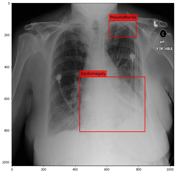
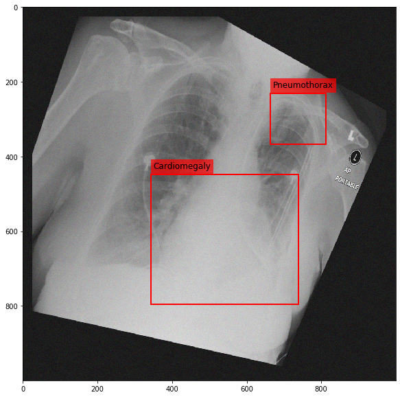
Visualizing the image

img = cv2.imread(os.path.join('Data', 'CXR', 'images', img_name))

fig = plt.figure(figsize=(10, 10))
ax = fig.add_subplot(1,1,1)
ax.imshow(img, cmap=plt.cm.Greys_r)

text_bbox = dict(facecolor='red', alpha=0.7, lw=0)
for _, entry in df.iterrows():
    ax.add_patch(Rectangle((entry.x, entry.y), entry.w, entry.h, fill=False, color='r', lw=2))
    ax.text(entry.x+6, entry.y-15, entry.finding,fontsize=12, bbox=text_bbox)
plt.show()

Creating a data container with the image, keypoints and the labels

We will encode Cardiomegaly as 0 and Pneumothorax as 1. In our case it is the first and the second rows respectively:

df

	Image Index	y	w	x	h	finding	img_present
202	00000732_005.png	464.000000	412.203390	427.932203	344.949153	Cardiomegaly	True
918	00000732_005.png	110.686823	172.942222	613.831111	103.537778	Pneumothorax	True

In SOLT, we decided to not implement separate class of augmentations for bounding boxes. Instead, we implemented all teh transformations for keypoints and thus we can just convert the bboxes into 4 keypoints:

pts = df[['x', 'y', 'w', 'h']].values
p1 = pts[:, :2].copy() # left top

p2 = pts[:, :2].copy()  # right top
p2[:, 0] += pts[:, 2]

p3 = pts[:, :2].copy()  # right bottom
p3[:, 0] +=  pts[:, 2]
p3[:, 1] +=  pts[:, 3]

p4 = pts[:, :2].copy()  # left bottom
p4[:, 1] +=  pts[:, 3]


cardiomegaly_kpts = solt.Keypoints(np.vstack((p1[0], p2[0], p3[0], p4[0])), img.shape[0], img.shape[1])
pneumothorax_kpts = solt.Keypoints(np.vstack((p1[1], p2[1], p3[1], p4[1])), img.shape[0], img.shape[1])

cardiomegaly_kpts.data

array([[427.93220339, 464.        ],
       [840.13559322, 464.        ],
       [840.13559322, 808.94915254],
       [427.93220339, 808.94915254]])

Alright, now we were able to store the bbox as keypoints, we can create a data container

dc = solt.DataContainer((img, cardiomegaly_kpts, 0, pneumothorax_kpts, 1), 'IPLPL')

As you can see from the above cell, the DataContainer does not care about the order of the objects in it, thus, we just used the format:

• Image
• Keypoints
• Label
• Keypoints
• Label

Now, let’s implement a simple augmentation pipeline.

Augmentation stream

stream = solt.Stream([
    slt.Projection(
            solt.Stream([
                slt.Scale(range_x=(0.8, 1.1), p=1),
                slt.Rotate(angle_range=(-90, 90), p=1),
                slt.Shear(range_x=(-0.2, 0.2), range_y=None, p=0.7),
        ]),
        v_range=(1e-6, 3e-4), p=1),
    # Various cropping and padding tricks
    slt.Pad(1000, 'z'),
    slt.Crop(1000, crop_mode='c'),
    slt.Crop(950, crop_mode='r'),
    slt.Pad(1000, 'z'),
    # Intensity augmentations
    slt.GammaCorrection(p=1, gamma_range=(0.5, 3)),
    solt.SelectiveStream([
        solt.SelectiveStream([
            slt.SaltAndPepper(p=1, gain_range=0.01),
            slt.Blur(p=0.5, blur_type='m', k_size=(11,)),
        ]),
        slt.Noise(p=1, gain_range=0.5),
    ]),
])

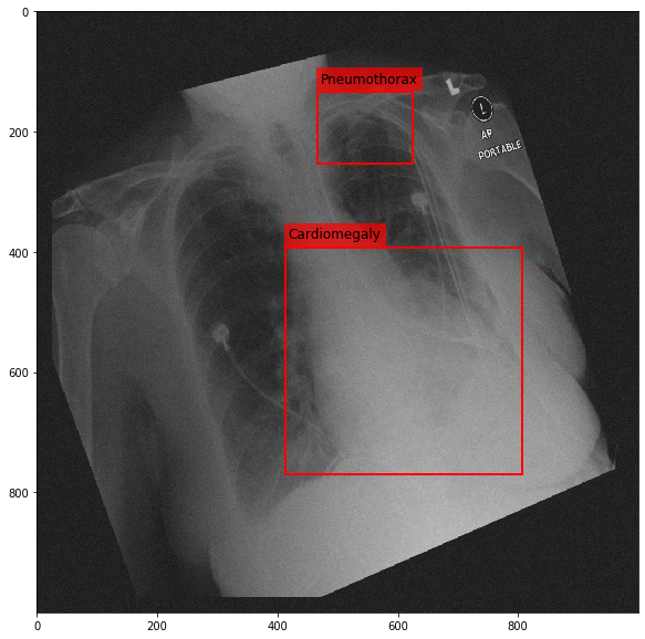
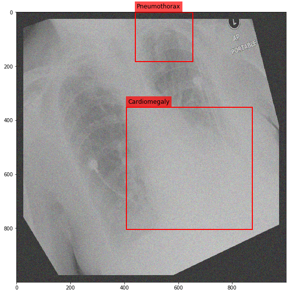
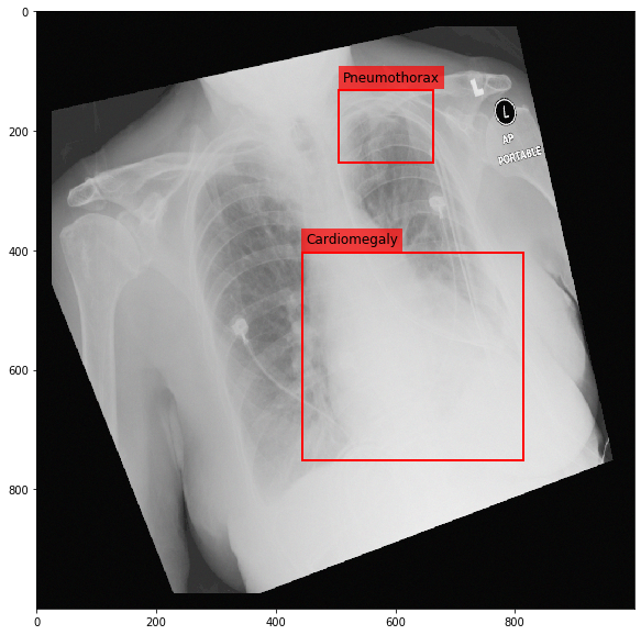
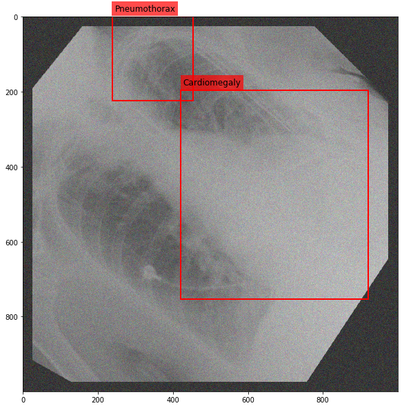
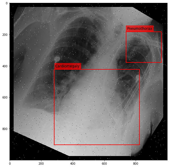
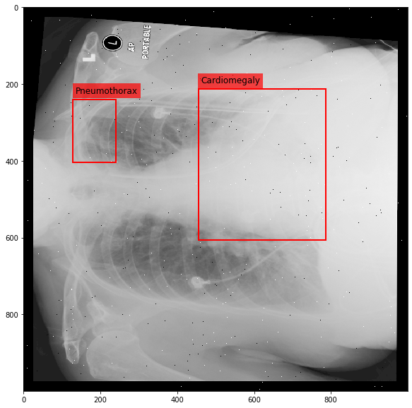
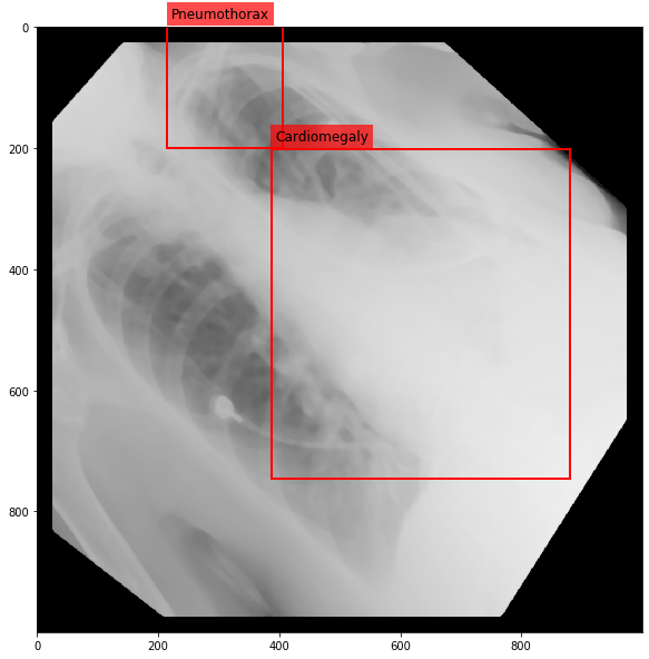
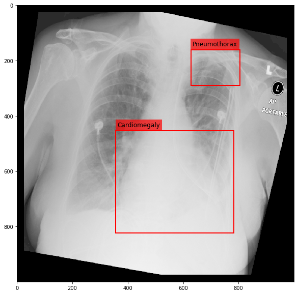
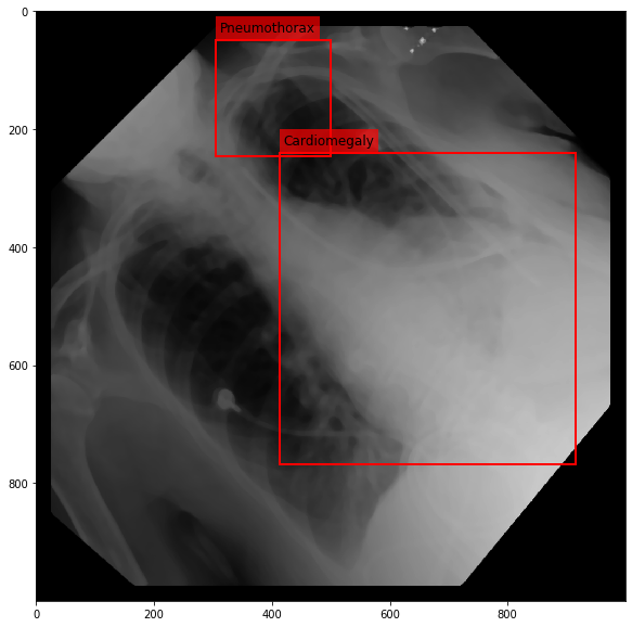
Augmenting a Chest X-ray

for i in range(10):
    res = stream(dc, return_torch=False)
    img_res, kp_c, lbl_c, kp_p, lbl_p = res.data
    fig = plt.figure(figsize=(10, 10))

    ax = fig.add_subplot(1,1,1)
    ax.imshow(img_res, cmap=plt.cm.Greys_r)

    for pts, cls in zip([kp_c.data, kp_p.data], ['Cardiomegaly', 'Pneumothorax']):
        text_bbox = dict(facecolor='red', alpha=0.7, lw=0)
        # Let's clip the points so that they will not
        # violate the image borders
        pts[:, 0] = np.clip(pts[:, 0], 0, img_res.shape[1]-1)
        pts[:, 1] = np.clip(pts[:, 1], 0, img_res.shape[0]-1)
        x, y = pts[:, 0].min(), pts[:, 1].min()
        w, h = pts[:, 0].max()-x, pts[:, 1].max()-y
        ax.add_patch(Rectangle((x, y), w, h, fill=False, color='r', lw=2))
        ax.text(x+6, y-15, cls, fontsize=12, bbox=text_bbox)
    plt.show()